Theoretical Foundation

What is credit risk and why is it important?

The likelihood that a borrower would not repay their loan to the lender ➔ the lenders will not receive their owned principle, moreover, they wouldn’t be paid the interest and will therefore suffer a substantial loss ➔ credit risk.
In addition, it is likely that the lender will have to sustain substaintial costs in an effort to recover outstanding debt ➔ collection costs.
When a borrower is not able to make the required payments to repay their debt ➔ default.

Some ways of lenders to protect themselves against credit losses:
• measure credit risk well,
• require collaterals,
• increase the price of lending the funds (the interest rate).

Expected loss (EL) and its components: PD, LGD and EAD

Expected loss is the amount a lender might lose by lending to a borrower.

EL = PD x LGD x EAD

Where:
PD – Probability of default: Brrowers inability to repat their debt in full or on time. PD is the estimate of the likelihood that the borrower would default. For the PD model, I need an indicator or a flag whether the borrower defaulted or not.
LGD – Loss given default: The proportion of the total exposure that cannot be recovered by the lender once a default has occured. LGD is the share of an asset that it lost if a borrower defaults. For the LGD model, I need to calculate how much of the loan was recovered after the borrower had defaulted. This information is contained in the recoveries column, so that will be our dependent variable.
EAD – Exposure at default: The total value that a lender is exposed to when a borrower default. EAD is the maximum that a bank may lose when a borrower defaults on a loan. For the EAD model, I must calculate the total exposure. At the moment the borrower defaulted compared to the total exposure in the past. You can find relevant information in the total recovered principle column. Of course I can use all other variables I have.

For example:
A borrower wants to buy a house: $500,000.
A bank funds 80% of a purchase, Loan-to-Value (LTV) = $500,000 x 80% = $400,000.
That borrower has to repay 10% = $400,000 x 10% = $40,000.
The outstanding balance = $400,000 – $40,000 = $360,000.
If the borrower defaults ➔ EAD = $360,000.
Assume that there is empirical evidence that one in four homeowners have defaulted in previous years. So PD = 1/4 = 25%.
If the borrowers defaults, the bank can sell the house immediately for $342,000 ➔ the bank can recover $342,000 ➔ the remaining loss = $360,000 – $342,000 = $18,000 ➔ LGD = $18,000/$360,000 = 5%.
➔ EL = PD x LGD x EAD = 25% x 5% x $360,000 = $45,000.

Capital adequacy, regulations, and the Basel II accord

To avoid all of things which could make economy paralyzed, regulators have come up with a set of rules that have two main goals:
(1) Regulate band operations and hence reduce risky behavior,
(2) Guarantee to the public that the banking system is in good health.

Capital requirement: Require banks to hold enough capital that would allow them to absorb the losses from defaults.
Capital adequacy ratio – CAR = Capital/Risk-Weighted assest >= 8%

The primary objective of the Basel II Accord is to ensure that the capital allocation bank carry out its risk sensitive. The greater the risk a bank is exposed to, the greater the amount of capital the bank needs to hold to safeguard its solvency and overall economic stability.
The three pillars of the Basel II Accord are:
(1) Minimum Capital Requirements,
(2) Supervisory Review,
(3) Market Discipline.

The three main types od risk banks face are:
(1) Credit Risk,
(2) Operational Risk,
(3) Market Risk

Basel II approaches: SA, F-IRB, and A-IRB

The Basel two accord prescribes that regulators should allow banks to choose from three different approaches for calculating or modeling credit risk.

That is, they can choose from one of three different approaches for calculating or modeling each of the three components of the expected loss. These three approaches are called Standardized Approach (SA), Foundation Internal Ratings Based approach (F-IRB), Advanced Internal Ratings Based approach (A-IRB).

Under the standardised approach, the capital that has to be held is prescribed as a percentage of the total exposure under the internal ratings based approaches. Expected loss, which is the product of PD, LGD, and EAD is calculated and the bank’s capital should be sufficient to cover expected losses.
Under the standardized approach, banks are required to use data from external credit agencies to assess credit risk.
The other two approaches are called internal ratings based because the standardized approach relies entirely on external ratings provided by credit agencies such as Fico, credit score for individuals and households. Other similar agencies are S&P, Moody’s and Fitch.

Presenting information about credit risk: The credit risk of every entity is represented by its Credit Rating. The lower the entity’s credit rating, the higher its credit risk. And hence one can infer that the entity has a low credit worthiness. For individuals, these credit ratings come in the form of credit scores. The most popular credit score is perhaps the Fico score. This is the credit score calculated and provided by a company called Fico. You may have heard that everyone has a Fico score, at least in the US. The score ranges between 300 and 850.

Please visit this link to calculate the FICO score of a borrower.

For firms, financial institutions and countries. Credit ratings are shown as letters. A good example is the S&P credit rating scale. The entities with the lowest credit risk and highest credit worthiness are rated as triple-A, and the ones with the highest credit risk and the lowest credit worthiness are rated with a D.

	SA	F-IRB	A-IRB
Probability of Default	Externally provided	Internally estimated	Internally estimated
Loss Given Default	Externally provided	Externally provided	Internally estimated
Exposure At Default	Externally provided	Externally provided	Internally estimated

IRB approaches:
• allow banks to establish their own credit ratings,
• precise calculations about the held capital for each individual exposure,
• allocate resources to cover losses.

Different facility types (asset classes) and credit risk modeling approaches

Under the standardized approach, particular types of borrowers and products are being treated in a different manner in terms of capital requirement calculations.For instance, I saw on one hand that the equivalent of 20% of the exposure towards every company rated from triple A to AA minus has to be held as capital. 50% of the exposure towards every company rated from A+ to a minus has to be held as capital and so on. On the other hand, for retail exposures of individuals, banks have to hold as much as 75% of capital of each exposure, and for mortgages, as much capital as 35% of each exposure.

As you can see, there are different approaches and rates to calculate capital requirements depending on what the borrower is a company, a corporation, another financial institution or a country.

The calculations also differ by product types, also called facility types. Even if the borrowers are of the same type, for example, both retail loans and mortgages are given to individuals, but retail exposures have a 75% weight, and mortgages have a 35% rate. Similarly, the internal ratings based IRB approaches may use different methods and statistical models for different types of borrowers and facility types.

Application model: Application models are used to estimate a firm’s credit rating at the moment of application. The estimated credit ratings in turn, are the basis on which banks decide whether to grant a loan or not. A bank may also use the estimated credit ratings to decide how to price the loan. That is what interest rate to charge for the respective loan. This is known as risk based pricing. The riskier a loan is, the higher will be its price, the higher the interest rate charged to the customer.

Behavior model: Behavioral models, on the other hand, are used to calculate probability of default and respectively expected loss after a loan is granted. Banks may also use behavioral models to decide whether to grant an additional loan to an existing customer.

---

Data

Introduction

Download dataset here.
The dataset contains all available data for more than 800,000 consumer loans issued from 2007 to 2015 by Lending Club: a large US peer-to-peer lending company. There are several different versions of this dataset. I have used a version available on kaggle.com. You can find it here:

Depending on the type of data, discrete or continuous, I will have to apply different pre-processing techniques. For our purposes, we’ll distinguish between two types discrete and continuous:
Discrete or categorical variables take only a certain finite number of values.
Continuous or numerical variables, on the other hand, can take any value in a given range, or in other words, they can take on an infinite number of possible values.

Fist, look at the columns and their descriptions:

and data columns’ infomation:

loan_data.info()

#	Columns	Non-Null Count	Dtype
0	Unnamed: 0	466285 non-null	int64
1	id	466285 non-null	int64
2	member_id	466285 non-null	int64
3	loan_amnt	466285 non-null	int64
4	funded_amnt	466285 non-null	int64
5	funded_amnt_inv	466285 non-null	float64
6	term	466285 non-null	object
7	int_rate	466285 non-null	float64
8	installment	466285 non-null	float64
9	grade	466285 non-null	object
10	sub_grade	466285 non-null	object
11	emp_title	438697 non-null	object
12	emp_length	445277 non-null	object
13	home_ownership	466285 non-null	object
14	annual_inc	466281 non-null	float64
15	verification_status	466285 non-null	object
16	issue_d	466285 non-null	object
17	loan_status	466285 non-null	object
18	pymnt_plan	466285 non-null	object
19	url	466285 non-null	object
20	desc	125981 non-null	object
21	purpose	466285 non-null	object
22	title	466264 non-null	object
23	zip_code	466285 non-null	object
24	addr_state	466285 non-null	object
25	dti	466285 non-null	float64
26	delinq_2yrs	466256 non-null	float64
27	earliest_cr_line	466256 non-null	object
28	inq_last_6mths	466256 non-null	float64
29	mths_since_last_delinq	215934 non-null	float64
30	mths_since_last_record	62638 non-null	float64
31	open_acc	466256 non-null	float64
32	pub_rec	466256 non-null	float64
33	revol_bal	466285 non-null	int64
34	revol_util	465945 non-null	float64
35	total_acc	466256 non-null	float64
36	initial_list_status	466285 non-null	object
37	out_prncp	466285 non-null	float64
38	out_prncp_inv	466285 non-null	float64
39	total_pymnt	466285 non-null	float64
40	total_pymnt_inv	466285 non-null	float64
41	total_rec_prncp	466285 non-null	float64
42	total_rec_int	466285 non-null	float64
43	total_rec_late_fee	466285 non-null	float64
44	recoveries	466285 non-null	float64
45	collection_recovery_fee	466285 non-null	float64
46	last_pymnt_d	465909 non-null	object
47	last_pymnt_amnt	466285 non-null	float64
48	next_pymnt_d	239071 non-null	object
49	last_credit_pull_d	466243 non-null	object
50	collections_12_mths_ex_med	466140 non-null	float64
51	mths_since_last_major_derog	98974 non-null	float64
52	policy_code	466285 non-null	int64
53	application_type	466285 non-null	object
54	annual_inc_joint	0 non-null	float64
55	dti_joint	0 non-null	float64
56	verification_status_joint	0 non-null	float64
57	acc_now_delinq	466256 non-null	float64
58	tot_coll_amt	396009 non-null	float64
59	tot_cur_bal	396009 non-null	float64
60	open_acc_6m	0 non-null	float64
61	open_il_6m	0 non-null	float64
62	open_il_12m	0 non-null	float64
63	open_il_24m	0 non-null	float64
64	mths_since_rcnt_il	0 non-null	float64
65	total_bal_il	0 non-null	float64
66	il_util	0 non-null	float64
67	open_rv_12m	0 non-null	float64
68	open_rv_24m	0 non-null	float64
69	max_bal_bc	0 non-null	float64
70	all_util	0 non-null	float64
71	total_rev_hi_lim	396009 non-null	float64
72	inq_fi	0 non-null	float64
73	total_cu_tl	0 non-null	float64
74	inq_last_12m	0 non-null	float64

---

Hypothesis

The below list is my questioning and provable hypotheses:

1. Higher grades (e.g., grade:A) significantly increase the likelihood of a positive outcome compared to the baseline grade.
2. Homeowners with a mortgage are more likely to achieve a positive outcome compared to renters.
3. Individuals with 10+ years of employment experience are more likely to achieve a positive outcome compared to those with less experience.
4. Lower interest rates significantly increase the likelihood of a positive outcome compared to higher interest rates.
5. Lower DTI values (e.g., 1.4-3.5) positively influence the likelihood of a positive outcome.
6. Individuals with longer credit histories (e.g., more than 271 months) are more likely to achieve a positive outcome.

EDA

Employment Length for Issued Loans:

Longer employment tenure (10+ years) correlates with the highest number of loans, while very short and moderate lengths show notable but lower issuance.

Payment Loan – Loan Amount:

• For target 0, the loan amounts with payment plans (y) have a broader distribution and higher density in the upper range compared to those without payment plans (n), which are more concentrated in the lower range.
• For target 1, the distribution of loan amounts is narrower overall, with payment plans (y) showing higher density at lower loan amounts, while those without payment plans (n) have a more uniform spread.

Amount and Status of Loans

• Fully Paid loans tend to have the largest range of loan amounts, with some outliers reaching very high values (around 35,000).
• Charged Off loans have a narrower range compared to Fully Paid, with most loans clustered around mid-to-high amounts.
• Loans in the Current and Default statuses exhibit relatively uniform ranges, with medians located slightly lower than Fully Paid loans.
• Late payment statuses (16–30 days and 31–120 days) and In Grace Period loans show similar ranges but lower overall loan amounts compared to Fully Paid or Charged Off categories.
• Loans labeled as Does not meet the credit policy are split into two groups (Fully Paid and Charged Off), with their distributions closely resembling their respective main categories.

Frequency of Grade of Loans

• Most of the loans are graded B, C and D.
• Grades E, F, and G have significantly lower counts, indicating they are less common in the dataset. This suggests a skew towards higher loan volume in the mid-tier grades (B, C, D).

Interest Rate Distribution

• For target = 0, the interest rates have a higher density in the range of approximately 12% to 15%, showing a sharper peak and a more concentrated distribution.
• For target = 1, the interest rates are more evenly distributed, with a broader density peak between 15% and 20%, suggesting higher variability compared to target = 0.

Interest Rate and Grade of Loans

• For each grade, the distributions for target = 0 and target = 1 are generally similar, with slight differences in density and spread.
• Grades A and B have the narrowest interest rate ranges (concentrated below 10%), while grades F and G exhibit the widest ranges and highest rates (extending beyond 25%).
• The spread for higher grades (F and G) is larger, suggesting more variability in interest rates, with noticeable overlap between target = 0 and target = 1.

Number of Loans by States

In the majority of states, non-defaulted loans outweigh defaulted ones, with only a small number of states where defaulted loans are comparable to or slightly higher than non-defaulted loans. This indicates a general trend of non-defaulted loans dominating across most states.

Median loan amounts are fairly consistent nationwide. However, Alaska (AK) exhibit greater variability in loan amounts, as indicated by longer whiskers and more outliers. The majority of loan amounts fall within a similar range across states, but outliers—represented as dots outside the whiskers—highlight occasional unusually high or low loan amounts in some states.

Loan Amount vs. Employment Length by Default or Non-Default

• Loan amounts are generally higher for target = 0 (non-defaulted loans) across all employment lengths, with the widest ranges and highest medians seen for borrowers with 10+ years of experience.
• Defaulted loans (target = 1) exhibit greater variability in the mid-range employment lengths (5-9 years), while borrowers with less than 1 year of experience tend to have the smallest loan amounts.

Loan Amount in each Term by Default or Non-Default

• For 36-month terms, loan amounts are generally smaller, with target = 0 (non-defaulted loans) having a slightly higher median and narrower range compared to target = 1 (defaulted loans).

• For 60-month terms, loan amounts are larger overall, with both target = 0 and target = 1 showing similar medians but with greater variability and more outliers in the target = 1 group.

Loan Amount in each Purposes with Default or Non-Default

• Purposes like “small business,” “house,” and “car” have higher median loan amounts and wider ranges, particularly for defaulted loans (target = 1), which often show greater variability and more outliers.
• Lower loan amounts are associated with purposes such as “educational,” “vacation,” and “moving,” where the distributions for target = 0 (non-defaulted loans) are generally tighter and show smaller ranges compared to target = 1.

Loan Amount in Initial List Status by and Target

• The distributions of loan amounts are similar, with slightly higher medians for non-defaulted loans (target = 0) compared to defaulted loans (target = 1).
• Both statuses exhibit comparable ranges and variability, with no significant differences between the two categories.

Loan Amount with Annual Income

• Most borrowers have annual incomes below USD100,000, with loan amounts distributed across a wide range, indicating that lower-income borrowers frequently take loans of varying sizes.
• There is a noticeable density of data points at the lower end of the annual income axis, suggesting a high concentration of lower-income borrowers.

• The majority of borrowers have a loan-to-income ratio between 0.1 and 0.3, making up 10% to 30% of their annual income.
• The density curve overlaid on the histogram highlights a peak around 0.2.
• Very few borrowers have a ratio above 0.4.

---

Data Preprocessing

Continuous variables Preprocessing

Emp_length: Employment length in years

loan_data['emp_length'].unique()

array(['10+ years', '< 1 year', '1 year', '3 years', '8 years', '9 years',
       '4 years', '5 years', '6 years', '2 years', '7 years', nan],
      dtype=object)

We need to remove the word ‘year’, ‘years’, ‘+ years’ after the number 1…10 by str.replace.

Earliest_cr_line: The month the borrower’s earliest reported credit line was opened

loan_data['earliest_cr_line']

We need to convert the categorical dates to numeric values by pd.to_datetime(). And the calculate the duration between the date of earliest_cr_line and the date I run the model.

Term: The number of payments on the loan

loan_data['term']

Remove the word ‘months’ to convert data to numeric values by pd.to_numeric(loan_data['term'].str.replace(' months', ''))

Issue_d: The month which the loan was funded

loan_data['issue_d']

Convert it to numeric dates by pd.to_datetime(loan_data['issue_d'], format = '%b-%y') and calculate the duration between it and the day I run the model.

Discrete variables processing

Grade: LC assigned loan grade

loan_data['grade'].value_counts()

Create dummy variables by pd.get_dummies(loan_data['grade'], prefix = 'grade', prefix_sep = ':').

Sub_grade: LC assigned loan subgrade

loan_data['sub_grade'].value_counts()

Creating dummy variables by pd.get_dummies(loan_data['sub_grade'], prefix = 'sub_grade', prefix_sep = ':').

Home_ownership: The home ownership status provided by the borrower during registration

loan_data['home_ownership'].value_counts()

Create dummy variables by pd.get_dummies(loan_data['home_ownership'], prefix = 'home_ownership', prefix_sep = ':').

Verification_Status: Indicates if the co-borrowers’ joint income was verified by LC, not verified, or if the income source was verified

loan_data['verification_status'].value_counts()

Create dummy variables by pd.get_dummies(loan_data['verification_status'], prefix = 'verification_status', prefix_sep = ':').

Loan_Status: Current status of the loan

loan_data['loan_status'].value_counts()

Create dummy variables by pd.get_dummies(loan_data['loan_status'], prefix = 'loan_status', prefix_sep = ':').

Purpose: A category provided by the borrower for the loan request

loan_data['purpose'].value_counts()

Create dummy variables by pd.get_dummies(loan_data['purpose'], prefix = 'purpose', prefix_sep = ':').

Addr_State: The state provided by the borrower in the loan application

loan_data['addr_state'].value_counts()

Initial_list_status: The initial listing status of the loan

loan_data['initial_list_status'].value_counts()

Create dummy variables by pd.get_dummies(loan_data['initial_list_status'], prefix = 'initial_list_status', prefix_sep = ':').

Finally, concatenate dummy variables into the dataframe:

# Concatenating dummy variables into a DataFrame
loan_data_dummies = pd.concat([pd.get_dummies(loan_data['grade'], prefix='grade', prefix_sep=':'),
                      pd.get_dummies(loan_data['sub_grade'], prefix='sub_grade', prefix_sep=':'),
                      pd.get_dummies(loan_data['home_ownership'], prefix='home_ownership', prefix_sep=':'),
                      pd.get_dummies(loan_data['verification_status'], prefix='verification_status', prefix_sep=':'),
                      pd.get_dummies(loan_data['loan_status'], prefix='loan_status', prefix_sep=':'),
                      pd.get_dummies(loan_data['purpose'], prefix='purpose', prefix_sep=':'),
                      pd.get_dummies(loan_data['addr_state'], prefix='addr_state', prefix_sep=':'),
                      pd.get_dummies(loan_data['initial_list_status'], prefix='initial_list_status', prefix_sep=':')],
                     axis=1)

Missing values checking and cleaning

total_rev_hi_lim: Total revolving high credit/credit limit

I fill the missing values with the values of funded_amnt column.

loan_data['total_rev_hi_lim'].fillna(loan_data['funded_amnt'], inplace=True)

annual_inc: The self-reported annual income provided by the borrower during registration

I fill the missing values with the mean of that column.

loan_data['annual_inc'].fillna(loan_data['annual_inc'].mean(), inplace=True)

mths_since_earliest_cr_line

I fill the missing values with the value of 0.

loan_data['mths_since_earliest_cr_line'].fillna(0, inplace=True)

acc_now_delinq: The number of accounts on which the borrower is now delinquent

I fill the missing values with the value of 0.

loan_data['acc_now_delinq'].fillna(0, inplace=True)

total_acc: The total number of credit lines currently in the borrower’s credit file

I fill the missing values with the value of 0.

loan_data['total_acc'].fillna(0, inplace=True)

pub_rec: Number of derogatory public records

I fill the missing values with the value of 0.

loan_data['pub_rec'].fillna(0, inplace=True)

open_acc: The number of open credit lines in the borrower’s credit file

I fill the missing values with the value of 0.

loan_data['open_acc'].fillna(0, inplace=True)

inq_last_6mths:The number of inquiries in past 6 months (excluding auto and mortgage inquiries)

I fill the missing values with the value of 0.

loan_data['inq_last_6mths'].fillna(0, inplace=True)

delinq_2yrs: The number of 30+ days past-due incidences of delinquency in the borrower’s credit file for the past 2 years

I fill the missing values with the value of 0.

loan_data['delinq_2yrs'].fillna(0, inplace=True)

emp_length_int: Employment length in years

I fill the missing values with the value of 0.

loan_data['emp_length_int'].fillna(0, inplace=True)

Model

PD Model

Data preparation

Dependent Variable: Good/ Bad (Default) Definition – Default and Non-default Accounts

loan_data['loan_status'].value_counts()

Calculate the proportion of each loan_status over the total number of observations:

loan_data['loan_status'].value_counts() / loan_data['loan_status'].count()

Next, I define the good/bad borrowers whose loan are ‘changred off’, ‘default’, ‘not meet the credit policy. Status: charged off’, and ‘Late (30-120 days)’ will be seen as 0 (bad), otherwise 1 (good).

loan_data['good_bad'] = np.where(loan_data['loan_status'].isin([
'Charged Off', 
'Default', 
'Does not meet the credit policy. Status:Charged Off', 
'Late (31-120 days)']), 0, 1)

I count the number of good and bad borrowers:

loan_data['good_bad'].value_counts()

Spliting the dataset into four dataframes:Inputs – Train, Inputs – Test, Targets – Train, Targets – Test after removing ‘good_bad’ dependent variable out of the dataset 80% of tha dataset will be used for training, 20% will be used for testing.

loan_data_inputs_train, loan_data_inputs_test, loan_data_targets_train, loan_data_targets_test = train_test_split(loan_data.drop('good_bad', axis = 1), loan_data['good_bad'], test_size = 0.2, random_state = 42)

I use the below codes to assign loan_data_inputs_train and loan_data_targets_train to two new dataframes df_inputs_prepr and df_targets_prepr in order to further data processing before reaching PD model compution.

df_inputs_prepr = loan_data_inputs_train
df_targets_prepr = loan_data_targets_train

After running the code df_inputs_prepr['grade'].unique(), I get the result:
array([‘C’, ‘E’, ‘A’, ‘D’, ‘B’, ‘F’, ‘G’], dtype=object),
then I concatenate it with the dataframe df_targets_prepr by the below code:

df_independent_vars = pd.concat([df_inputs_prepr['grade'], df_targets_prepr], axis = 1) # Concatenating two dataframes along the columns.
df_independent_vars.head()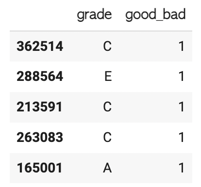

I group the data by counting the observations of each grade:

df_independent_vars.groupby(
df_independent_vars.columns.values[0], as_index = False)[df_independent_vars.columns.values[1]].count()

Weight of Evidence

The Weight of Evidence (WOE) tells the predictive power of an independent variable in relation to the dependent variable. Since it evolved from credit scoring world, it is generally described as a measure of the separation of good and bad customers.
• “Bad Customers” refers to the customers who defaulted on a loan, and
• “Good Customers” refers to the customers who paid back loan.

where,
• Distribution of Goods – % of Good Customers in a particular group,
• Distribution of Bads – % of Bad Customers in a particular group,
• ln – Natural Log,
• Positive WOE means Distribution of Goods > Distribution of Bads,
• Negative WOE means Distribution of Goods < Distribution of Bads

df_independent_vars['WoE'] = np.log(df_independent_vars['proportion_numbers_of_good'] / df_independent_vars['proportion_numbers_of_bad'])

Information Value

IV (Information Value) and WOE are closely related. IV is a data exploration technique that helps determine which variable in a data set has predictive power or influence on the value of a specified dependent variable (0 or 1).

IV is a numerical value that quantifies the overall predictive strength of an independent variable X in capturing the binary dependent variable Y and is defined mathematically as the sum of the absolute values for WOE across all groups.

IV is helpful for reducing the number of variables used for building a Logistic Regression model, especially when there are many potential variables. IV analyzes each individual independent variable in turn without considering other predictor variables. Based on the IV values of the variable, I use the below logic to understand its predictive power:

Logistic Regression

Estimate the coefficients of the object from the ‘LogisticRegression’ class with inputs (independent variables) contained in the first dataframe and targets (dependent variables) contained in the second dataframe.

reg = LogisticRegression()
reg.fit(inputs_train, loan_data_targets_train)

I also calculate p-values and add to the summary table:

PD Model Validation

ROC & AUROC

A receiver operating characteristic (ROC) curve is a graph that shows how well a binary classifier model performs at different threshold values. It plots the true positive rate (TPR) against the false positive rate (FPR) at each threshold setting.

The ROC curve is a useful tool for comparing the performance of different classifiers and determining if a classifier is better than random guessing. The position of the ROC curve on the graph reflects the accuracy of the diagnostic test. 

The area under the ROC curve (AUC) is a common performance metric for an ROC curve. The value of the AUC should be as large as possible within the range of zero to one.

Calculate the Area Under the Receiver Operating Characteristic Curve (AUROC) from a set of actual values and their predicted probabilities:

A common scale for the area under the ROC curve.
• The model is Bad if its area under the curve is between 50% and 60%.
• If it is between 60% and 70%, the model is fair.
• If it is between 70% and 80%, the model is good.
• If it is between 80% and 90%, the model is excellent.

AUROC = roc_auc_score(df_actual_predicted_probs['loan_data_targets_test'], df_actual_predicted_probs['y_hat_test_proba'])
print(f"The area under the curve is: {AUROC:.2%}")

The area under the curve is: 70.18% → the model is good.

Gini and Kolmogorov-Smirnov

Gini is created as a measure of income inquality, or to measure the inequality between the rich and the poor individuals. In credit risk modeling, Gini is utilized with the same purpose to measure inequality between non defaulted or good borrowers and defaulted or bad borrowers in a population.

The Gini coefficient is measured by plotting the cumulative proportion of defaulted or bad borrowers as a function of the cumulative proportion of all borrowers.

The Gini coefficient is the percentage of the area above the secondary diagonal line enclosed between this concave curve and the secondary diagonal line. The greater the area, the better the model.

Gini = AUROC * 2 - 1

0.40358843783278964

Kolmogorov-smirnov shows to what extent the model separates the actual good borrowers from the actual bad borrowers. It is measured by looking at the cumulative distributions of actual good borrowers and actual bad borrowers with respect to the estimated probabilities of being good and bad by our model.
Kolmogorov-smirnov or K-s, in short, is the maximum difference between the cumulative distribution functions of good and bad borrowers with respect to predicted probabilities. The greater this difference, the better the model.

Calculate KS from the data. It is the maximum of the difference between the cumulative percentage of ‘bad’ and the cumulative percentage of ‘good’.

KS = max(df_actual_predicted_probs['Cumulative Perc Bad'] - df_actual_predicted_probs['Cumulative Perc Good'])

0.2968539589918978

The Kolmogorov-Smirnov (KS) statistic of 0.2969 (approximately) represents the maximum separation between the cumulative distribution functions of the good and bad borrowers based on their estimated probability of being “good” as predicted by the model.

In practical terms, this KS value indicates how well the model discriminates between the two groups (good vs. bad borrowers). A higher KS value typically suggests a better model in terms of its ability to separate these groups; it means that the model’s predictions for good and bad borrowers are more distinct.
• Separation Ability: A KS value of 0.2969 implies that there is roughly a 29.69% maximum difference between the cumulative probability distributions for good and bad borrowers. This separation shows how well the model can distinguish between them.
• Model Quality: Generally, in credit scoring and binary classification contexts, a KS statistic above 0.3 is considered reasonably good, while values above 0.4 indicate strong discriminatory power. Since 0.2969 is close to 0.3, it suggests the model has moderate discriminatory power, but there could still be room for improvement.
• In the plot, this maximum difference corresponds to the largest vertical distance between the red (bad borrowers) and blue (good borrowers) lines. The larger this distance, the more effective the model is at correctly ranking borrowers by their likelihood of being good or bad.

Apply PD Model to calcuate Credit Score

FICO credit scores are a method of quantifying and evaluating an individual’s creditworthiness. FICO scores are used in 90% of mortgage application decisions in the United States.

Created by the Fair Isaac Corporation, FICO scores consider data in five areas: payment history, the current level of indebtedness, types of credit used, length of credit history, and new credit accounts.  A FICO score ranges from 300 to 850 and is categorized into five ranges:

Let try to calculate the Credit Score of the observation of 362514.
• The intercept = 342,
• Grade C (true) = 47,
• Home ownership – MORTGAGE = 9,
• address – CA = 6,
• verification_status:Verified is -1,
• purpose:major_purch__car__home_impr = 21,
• mths_since_issue_d:40-41 = 72,
• int_rate:12.025-15.74 = 31,
• mths_since_earliest_cr_line:165-247 = 5,
• inq_last_6mths:0 = 23,
• annual_inc:60K-70K = 10,
• dti:7.7-10.5 = 11,
• mths_since_last_delinq:Missing = 7,
• mths_since_last_record:Missing = 11.

Altogether = 594, is the credit score of the observation of 362514.

Credit Score to PD Model

Follow the several steps to calculate Score from my notebook, I eventually calcuate the number of rejected/approved applications, and the rate of these variables.

Some conclusions:
• With the cutoff level of 0.9, I will end up with 53.66% approval rate at about 46.34% rejection rate.
• With the probability of default of 5%, I have a 20.83% approval rate and a 79.16% rejection rate

df_cutoffs.head()

df_cutoffs.tail()

PD Model Monitoring

To monitor PD model, I use a different dataset named loan_data_2015.csv and assigned it under another name as: ‘loan_data’.

loan_data.head()

Similar to the original dataset, I also do some preprocessing methods to cleanse the data before being used to validate the PD model.

In this section, I will use Population Stability Index aka PSI. PSI is a measure of how much a population has shifted over time or between two different samples of a population in a single number. It does this by bucketing the two distributions and comparing the percents of items in each of the buckets, resulting in a single number you can use to understand how different the populations are. The common interpretations of the PSI result are:
• PSI >= 0.2: significant population change,
• PSI < 0.1: no significant population change,
• PSI < 0.2: moderate population change.

A formula to calculate PSI is:

PSI_calc.groupby('Original feature name')['Contribution'].sum().sort_values(ascending=True)

Based on the PSI scale, here are my conclusions:
• No Significant Population Change (PSI < 0.1): Features such as acc_now_delinq, addr_state, home_ownership, annual_inc, grade, and emp_length have a PSI contribution below 0.1, indicating no significant population change for these features. These features are stable, and there has been minimal change in the distribution of these variables between the compared datasets.
• Moderate Population Change (PSI ≈ 0.1 – 0.2): Features like term, mths_since_earliest_cr_line, inq_last_6mths, and verification_status fall within the range close to 0.1 or slightly higher, suggesting moderate population change. These features show some degree of change, but it’s not substantial enough to indicate a drastic shift.
• Significant Population Change (PSI ≥ 0.2): The features initial_list_status, Score, and mths_since_issue_d have contributions above 0.2, indicating a significant population change. In particular, mths_since_issue_d has the highest PSI contribution (2.388305), signaling a substantial shift in this variable’s distribution. This feature may need further investigation, as it suggests a significant change in the population structure related to the time since the loan was issued. Score and initial_list_status also indicate notable changes, which may affect the model’s predictive power if these shifts are not accounted for.

---

LGD and EDA Model

Loss given default (LGD) is the estimated amount of money a bank or other financial institution loses when a borrower defaults on a loan. LGD is depicted as a percentage of total exposure at the time of default or a single dollar value of potential loss. A financial institution’s total LGD is calculated after a review of all outstanding loans using cumulative losses and exposure.
Exposure at default is the total value of a loan that a bank is exposed to when a borrower defaults.  For example, if a borrower takes out a loan for $100,000 and two years later the amount left on the loan is $75,000, and the borrower defaults, the exposure at default is $75,000.

A common variation considers the exposure at risk and recovery rate. Exposure at default is an estimated value that predicts the amount of loss a bank may experience when a debtor defaults on a loan. The recovery rate is a risk-adjusted measure to right-size the default based on the likelihood of the outcome.
LGD (in dollars) = Exposure at Risk (EAD) * (1 – Recovery Rate)
where Recovery Rate = Recoveries / Funded Amount
(Source: https://www.investopedia.com/terms/l/lossgivendefault.asp)

loan_data_defaults['recovery_rate'] = loan_data_defaults['recoveries'] / loan_data_defaults['funded_amnt']

EAD is the predicted amount of loss a bank may be exposed to when a debtor defaults on a loan. Banks often calculate an EAD value for each loan and then use these figures to determine their overall default risk. There are two methods to determine exposure at default.
• Regulators use the first approach, which is called foundation internal ratings-based (F-IRB). This approach to determining exposure at risk includes forward valuations and commitment detail, though it omits the value of any guarantees, collateral, or security.
• The second method, called advanced internal ratings-based (A-IRB), is more flexible and is used by banking institutions. Banks must disclose their risk exposure. A bank will base this figure on data and internal analysis, such as borrower characteristics and product type. EAD, along with loss given default (LGD) and the probability of default (PD), are used to calculate the credit risk capital of financial institutions. (https://www.investopedia.com/terms/e/exposure_at_default.asp) In this notebook, I use the second method and the formula to calculate I use is:
EAD = Total Funded Amount x Credit Conversion Factor

To calculate credit conversion factor or CCF, in this case, I use the variables [‘fund_amt’], and [‘total_rec_prncp’]:

loan_data_defaults['CCF'] = (loan_data_defaults['funded_amnt'] - loan_data_defaults['total_rec_prncp']) / loan_data_defaults['funded_amnt']

I plot a histogram chart by the data [‘recovery_rate’] and [‘CCF’] to view the frequency and density of the variables by plt.hist:

plt.hist(loan_data_defaults['CFF'], bins = 100)

The two variables are proportions. They are constrained between 0 and 1.

Methodologically speaking, the density of proportions is best described as a specific distribution called beta distribution. The regression model used to assess the impact of a set of independent variables on a variable with beta distribution is called beta regression.

Normally it is used to model outcomes that are strictly greater than zero and strictly lower than one. However, some alterations allow for modeling outcomes that are greater than or equal to zero and lower than or equal to one, which is typically the case with recovery rate and credit conversion factor.

Currently there is no major Python library that supports a stable version of beta regression, therefore, finding an alternative is crucial. One possible solution is to use the functionalities of the other most popular statistical computing environment for data science are. Currently there are libraries in R that are capable of estimating beta regression models and I can write and run r code within python using packages such as r packages. But conversion of Python objects such as large data frames to r objects and vice versa may require a lot of random access memory. Due to these reasons, instead of the state of the beta regression models, applying simpler yet methodologically appropriate statistical models is still good.

plt.hist(loan_data_defaults['recovery_rate'], bins = 50)

It’s can be seen that about half of the observations have a recovery rate of zero, while the rest of recovery rates greater than zero.

So for estimating LGD, it’s plausible to have a two stage approach. First, to model whether the recovery rate is zero or not, that means zero or greater than zero then only if it’s greater than zero to model how much exactly it is. The first question is a binary question similar to the probability of default where I modeled if a borrower had defaulted or not. Here the recovery rate is zero or not, so using the same model logistic regression is good.

For this model, need to create a new binary dependent variable ‘recovery_zero_one’. It is zero when recovery rate is zero and one otherwise.

To summarize, to model LGD, building a logistic regression model to estimate whether the recovery rate is zero or is greater than zero. Then for accounts where recovery rate is greater than zero, using a linear regression model to estimate how much exactly it is.

LGD Model

Logistic Regression

LGD model in stage 1 datasets: recovery rate 0 or greater than 0. I split the data as the following codes:

lgd_inputs_stage_1_train, lgd_inputs_stage_1_test, lgd_targets_stage_1_train, lgd_targets_stage_1_test = train_test_split(loan_data_defaults.drop(['good_bad', 'recovery_rate','recovery_rate_0_1', 'CCF'], axis = 1), loan_data_defaults['recovery_rate_0_1'], test_size = 0.2, random_state = 42)

After running the code LogisticRegression_with_p_values(), I get the summary table:

I will calculate the Receiver Operating Characteristic (ROC) Curve from a set of actual values and their predicted probabilities.

I get three arrays: the false positive rates, the true positive rates, and the thresholds.

fpr, tpr, thresholds = roc_curve(df_actual_predicted_probs['lgd_targets_stage_1_test'], df_actual_predicted_probs['y_hat_test_proba_lgd_stage_1'])

I plot the false positive rate along the x-axis and the true positive rate along the y-axis, thus plotting the ROC curve.

plt.plot(fpr, tpr)
plt.plot(fpr, fpr, linestyle = '--', color = 'k')
plt.xlabel('False positive rate')
plt.ylabel('True positive rate')
plt.title('ROC curve')

I also calculate the Area Under the Receiver Operating Characteristic Curve (AUROC) from a set of actual values and their predicted probabilities.

AUROC = roc_auc_score(df_actual_predicted_probs['lgd_targets_stage_1_test'], df_actual_predicted_probs['y_hat_test_proba_lgd_stage_1'])

0.6479684167438654

Linear Regression

I Take only rows where the original recovery rate variable is greater than one, i.e. where the indicator variable I created is equal to 1.

lgd_stage_2_data = loan_data_defaults[loan_data_defaults['recovery_rate_0_1'] == 1]

The dataset of the LGD model stage 2 also has the same technique as that of stage 1:

gd_inputs_stage_2_train, lgd_inputs_stage_2_test, lgd_targets_stage_2_train, lgd_targets_stage_2_test = train_test_split(lgd_stage_2_data.drop(['good_bad', 'recovery_rate','recovery_rate_0_1', 'CCF'], axis = 1), lgd_stage_2_data['recovery_rate'], test_size = 0.2, random_state = 42)

I run the stage model 2 by LinearRegression() and get the result:

EAD Model

I prepare the data for running this model:

ead_inputs_train, ead_inputs_test, ead_targets_train, ead_targets_test = train_test_split(loan_data_defaults.drop(['good_bad', 'recovery_rate','recovery_rate_0_1', 'CCF'], axis = 1), loan_data_defaults['CCF'], test_size = 0.2, random_state = 42)

I run the EAD model by LinearRegression() and get the result:

---

Expected Loss

I calculate estimated EAD (Estimated EAD equals estimated CCF multiplied by funded amount):

loan_data_preprocessed['EAD'] = loan_data_preprocessed['CCF'] * loan_data_preprocessed_lgd_ead['funded_amnt']

Finally, I get the result:

loan_data_preprocessed_new[['funded_amnt', 'PD', 'LGD', 'EAD', 'EL']]

---