Tất cả những thao tác được liệt kê bên dưới đều nằm trong hộp thoại Format Cell, mở nhanh bằng tổ hợp phím Ctrl+1
All formatting methods shown below are available on Format Cell dialogue box, quickly open it by pressing Ctrl+1
#1: TIME – Thời gian
Excel quy ước như sau:
Some time abbreviations listed in the below table:
| Letter | Stands for | Display (ex: 07:05:03) |
| h | hour: giờ | h = 7, hh = 07 |
| m | minute: phút | m = 5, mm = 05 |
| s | second: giây | s = 3, ss = 03 |
Ngoài ra, Excel còn phân biệt AM (ante merīdiem) và PM (post merīdiem):
Khi nhập từ 00:00:00 đến 11:59:59, Excel mặc định là giờ AM và thời gian còn lại là PM.
Có 2 cách để nhập giờ PM:
– Cách 1: nhập giờ kiểu giờ 24 tiếng, ví dụ: 13:30:00,
– Cách 2: nhập giờ kiểu giờ 12 tiếng và chỉ cần thêm chữ p phía sau, ví dụ: 1:30 p
Additionally, users can display the time in AM/PM format. The duration between 00:00:00 and 11:59:59 is in the AM time, the rest of duration in one day is in the PM time.
Two ways to input PM time:
– Method 1: type the time under formatted 24 hours, ex: 13:30:00,
– Method 2: type the time under formatted 12 hours, add the letter p next to the time, ex: 1:30p
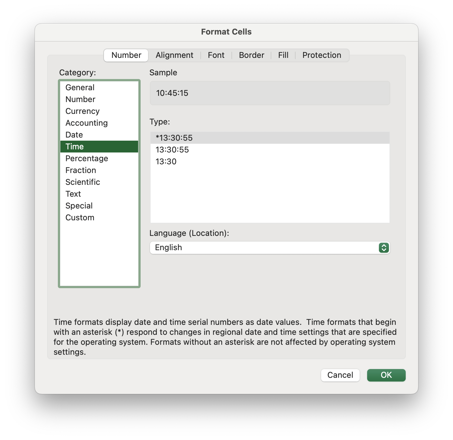
Xem thêm các định dạng cho giờ tại thẻ TIME:
More formats in TIME page:
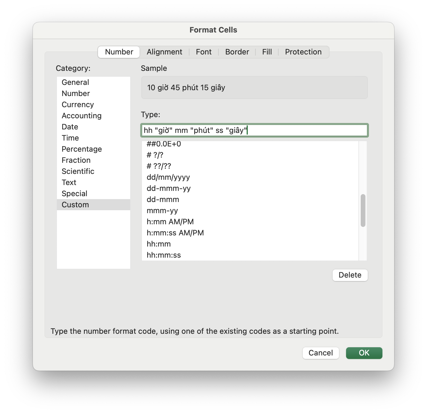
Nếu bạn muốn hiển thị chữ “giờ”, “phút”, “giây” thì nhập format này tại thẻ Custom:
If you want to show “hour”, “minute” and “second” at the right of the time, please input the following code in Custom:
#2: DATE – Ngày tháng
Excel quy ước như sau:
Some date abbreviations listed in the below table:
| Letter | Stands for | Display (ex: 02/09/2021) |
| d | day: ngày | d = 2, dd = 02, ddd = Thu, dddd = Thurday |
| m | month: tháng | m = 9, mm = 09, mmm = Sep, mmmm = September |
| y | year: năm | y = yy = 21, yyy = yyyy = 2021 |
Lưu ý khi nhập ngày tháng năm:
Tuỳ máy tính sẽ có format hiển thị ngày tháng năm khác nhau, ví dụ: 02/09/2021, 9/2/21, 2021/09/02,… Nên trước khi nhập dữ liệu, bạn lưu ý xem máy tính mình đang có định dạng như thế nào để nhập cho phù hợp.
Note:
Dates do not have the same formattings in systems, such as 02/09/2021, 9/2/21, 2021/09/02,… Therefore, before typing dates, please note what kind of date format is.
Hướng dẫn thay đổi hiển thị ngày tháng năm:
More – Some ways to change date format:
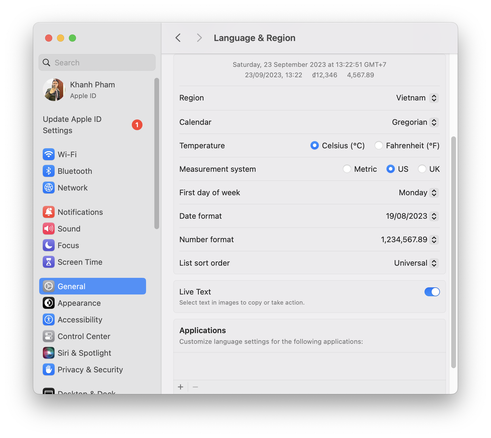
Đối với MacOS – For MacOS:
➤ System Preferences ➤ Language & Region ➤ Advanced ➤ Dates
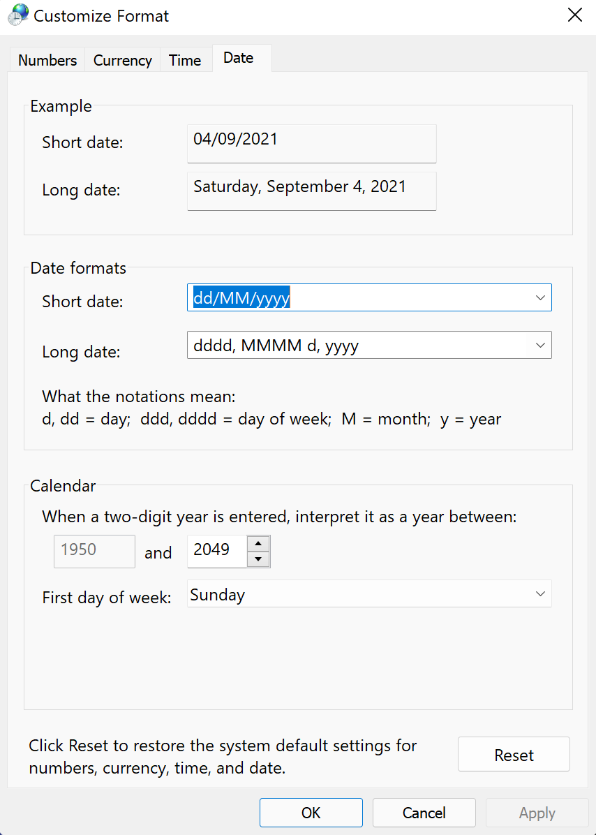
Đối với WinOS – For WinOS:
Control Panel ➤ View by Category: Change Date, Time or Number Format (below Clock and Region) ➤ Additional Settings ➤ Date
Khi nhập ngày tháng năm, để đảm bảo tính chính xác và đồng bộ, sử dụng hàm =DATE(năm,tháng,ngày).
To input date precisely and synchronously, please use the function =DATE(year,month,day).
Cách hiển thị thứ bằng nhiều ngôn ngữ khác nhau:
More – Display days of week in some languages:
Nhập mã bên dưới trước định dạng ngày:
Add the below code before day format:
| Tiếng Việt | [$-vi-VN] |
| Tiếng Trung | [$-zh-CN] |
| Tiếng Hàn | [$-ko-KR] |
| Tiếng Nhật | [$-ja-JP] |
| Tiếng Thái | [$-th-TH] |
Xem đầy đủ tất cả các quốc gia tại đây
Get more details here
#3: CURRENCY – Tiền tệ
Để hiển thị nhanh đơn vị tiền tệ, sử dụng nút lệnh $ ở nhóm lệnh Number:
To display numbers in currency format, use $ button in Number group:
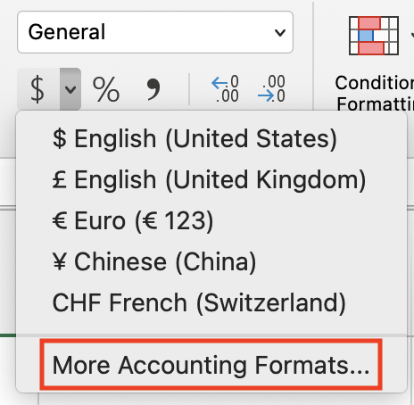
Để hiển thị những đồng tiền khác, chọn More Accounting Formats để mở thẻ ACCOUNTING:
To show other currencies, More Accounting Formats to access ACCOUNTING page:
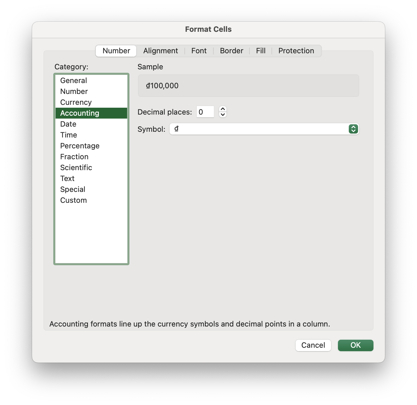
Trong đó – Where:
• Decimal Places: hiển thị phần thập phân,
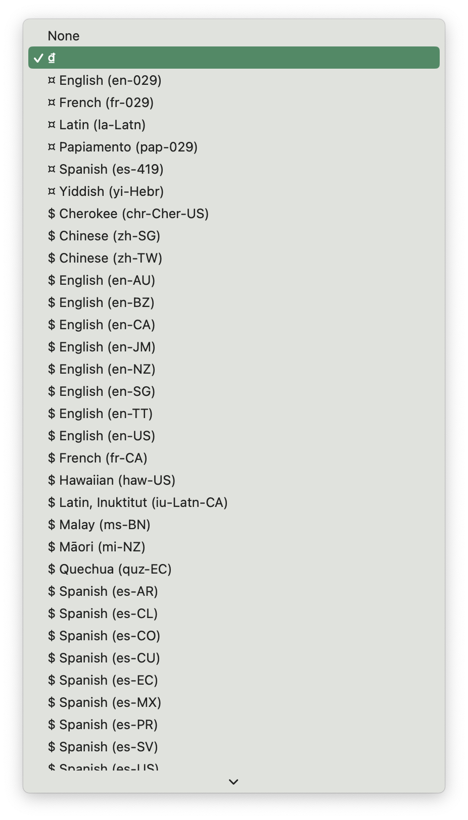
• Symbol: chọn đơn vị tiền tệ, (Việt Nam đồng là VND,…)
Hoặc ở thẻ CURRENCY:
Or in CURRENCY page:
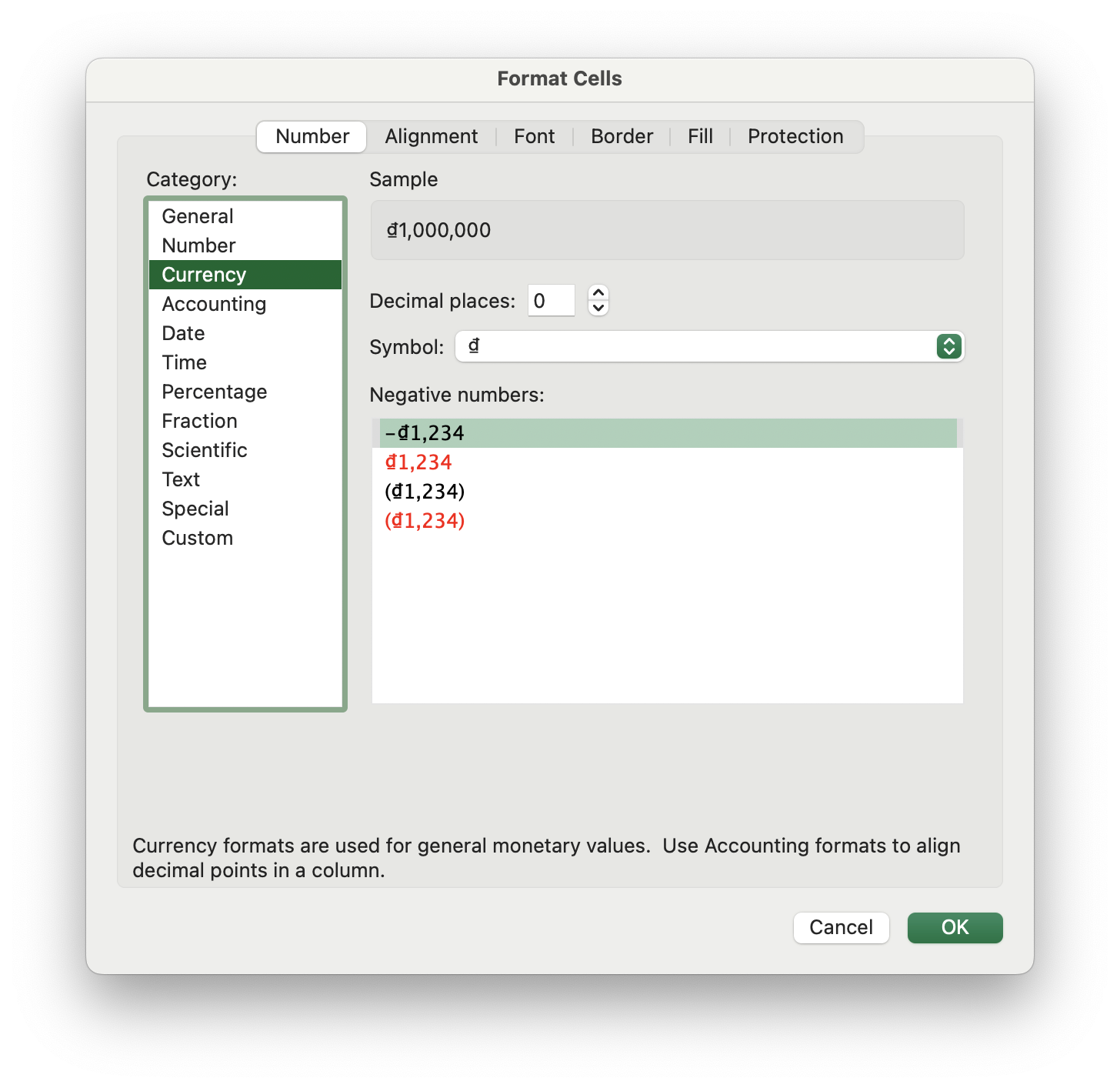
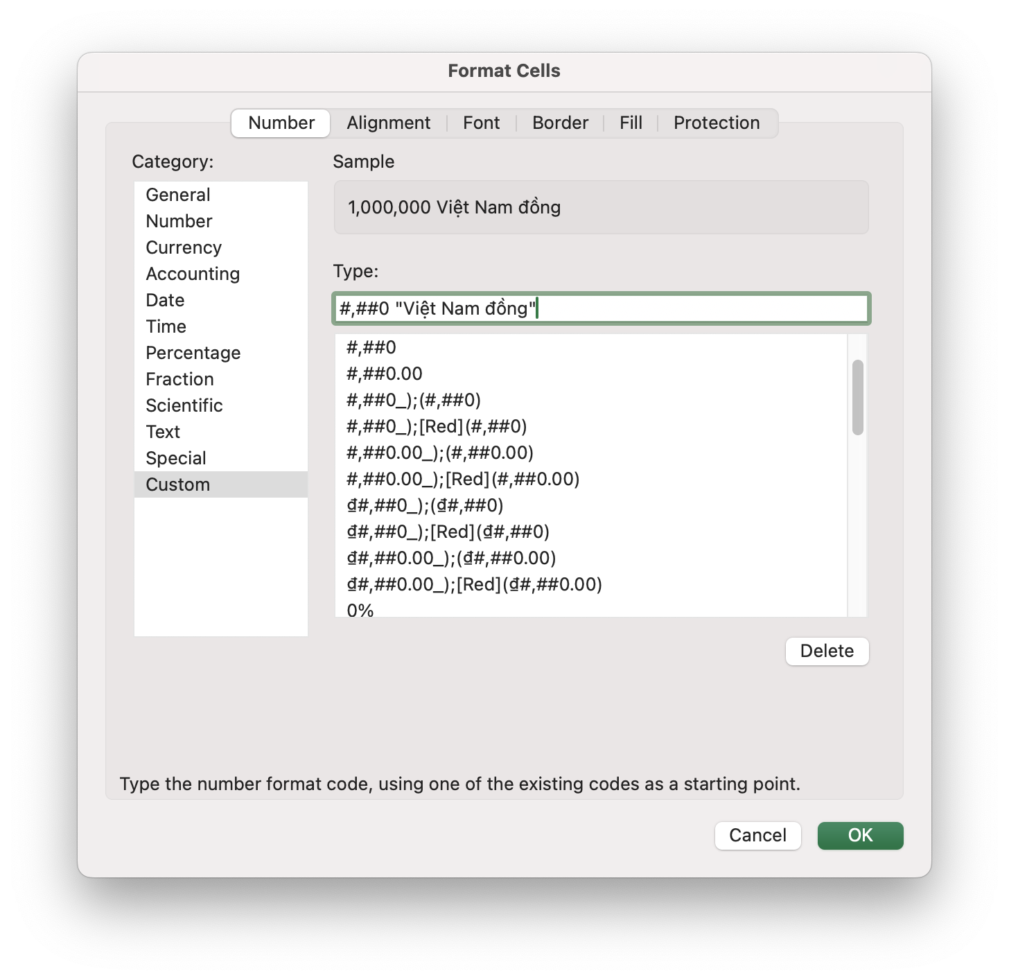
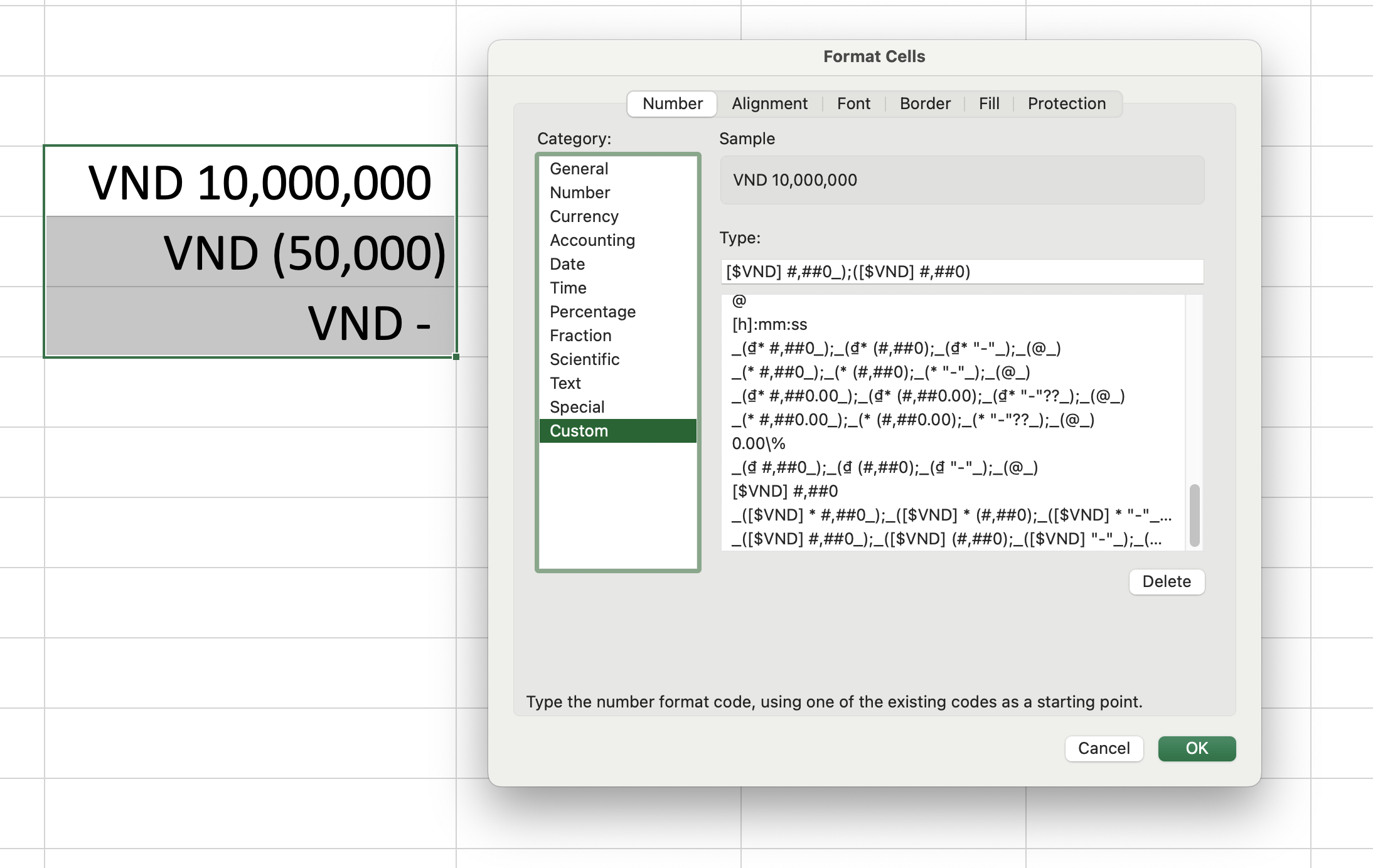
Vì đây là phiên bản quốc tế nên đơn vị tiền tệ như VND, USD, JPY, GBP đều nằm trước số tiền. Để hiển thị đơn vị tiền tệ ở phía sau số tiền, nhập format “đơn vị tiền tệ” tại Custom.
The Excel is an international app so that currency symbols are put the left numbers. To show currency symbols at the right of numbers, type as the following code in Custom page:
#4: FRACTION – Phân số
Excel mặc định không hiển thị phân số khi chúng ta nhập 0.2 hoặc 0.5.
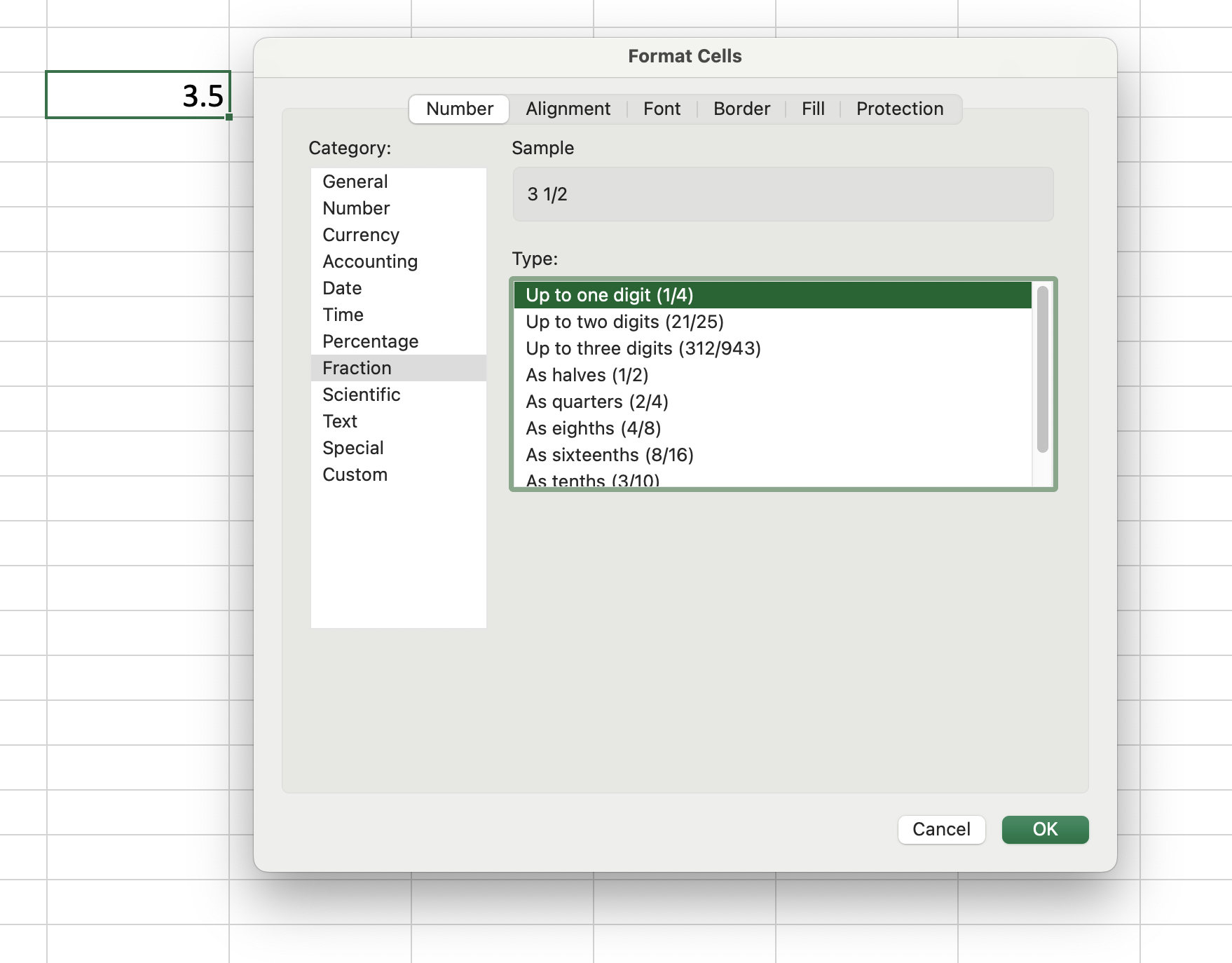
Sử dụng thẻ FRACTION để chuyển số thập phân thành phân số gần với nó nhất:
Excel basically does not support to convert a decimal to a fraction automatically when typing a decimal number. We can convert it at the FRACTION page:
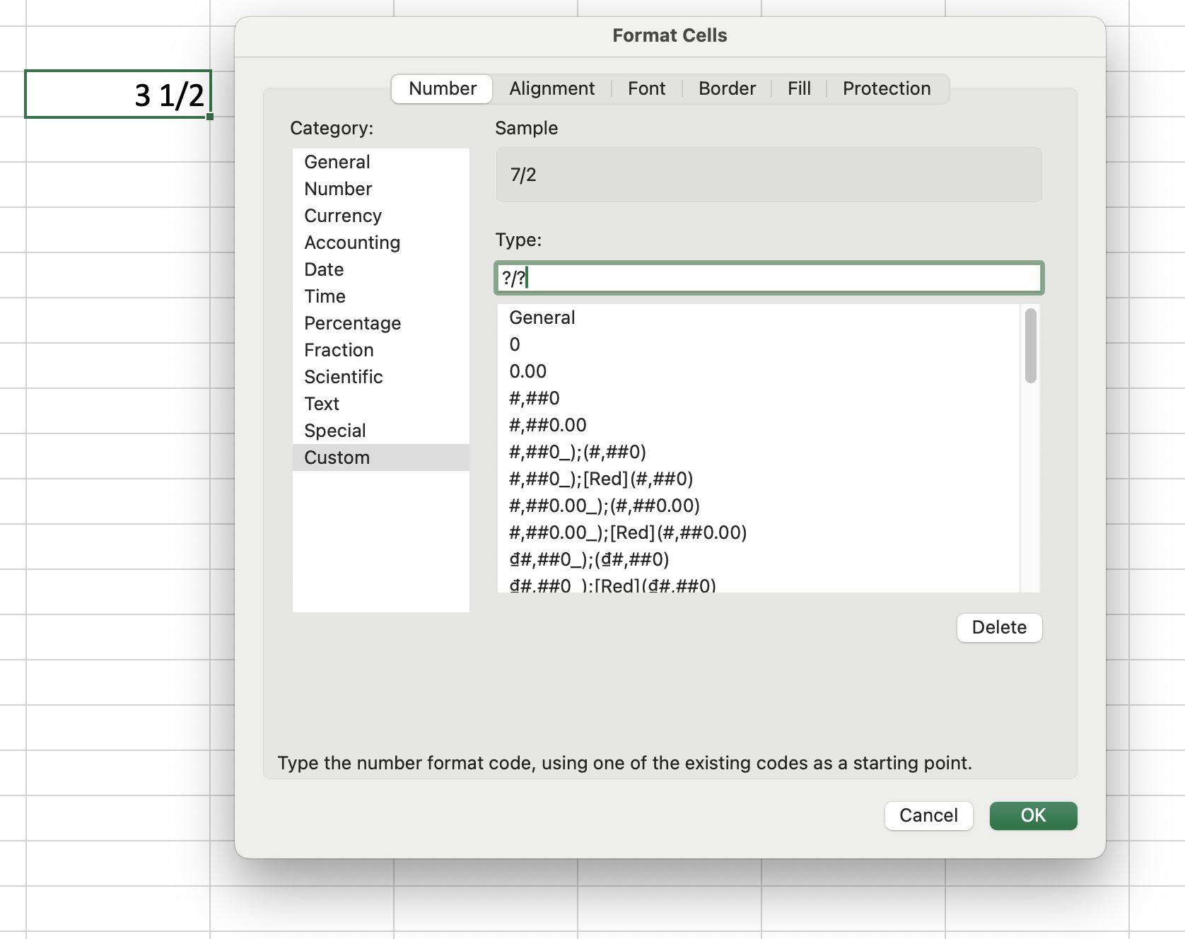
Để hiển thị dạng phân số thông thường, nhập ?/? hoặc 0/0 tại Custom:
Type ?/? or 0/0 in Custom Type: to show a normal fraction:
Để nhập và hiển thị phân phố, đặt số 0 phía trước phân số. Ví dụ, nếu muốn nhập và hiển thị 1/2, hãy nhập 0(phím cách)1/2. Excel sẽ bỏ đi số 0 và giữ nguyên định dạng phân số. Nếu nhập trực tiếp 1/2 vào ô, Excel sẽ xem đó là một ngày (1 tháng 2 hoặc 2 tháng 1).
To input and display a fraction, please put 0 (zero) before a fraction. For example, if you want to input and display a half in Excel, please type: 0(space)1/2. Excel will remove 0 before your fraction and keep fractional formatting, 1/2. You can not type 1/2 directly into a cell because Excel immediately identify your value as a date (1 February or 2 January).
Input: 0 14/5 → 2 4/5, 0 1/4 → 1/4, 1 1/2 → 1 1/2
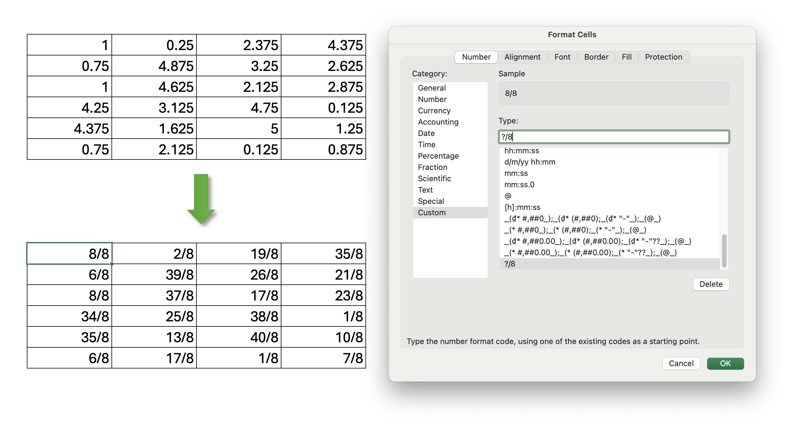
Để quy đồng mẫu số, tại custom, nhập #/mẫu số muốn quy đồng, ví dụ, #/8.
To share the same denominator, at custom, type #/denominator, #/8 for example.
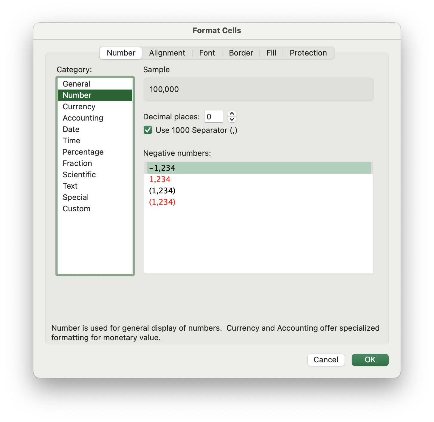
#5: NUMBER – Số
Thẻ NUMBER cho phép:
• Định dạng phân cách hàng nghìn,
• Tuỳ chỉnh tăng/giảm phần thập phân, và
• Hiển thị số âm.
At the NUMBER page, users can:
• Format a number as comma style (checkbox: Use 1000 Separator),
• Increase or decrease the decimal places, and
• Display negative numbers.
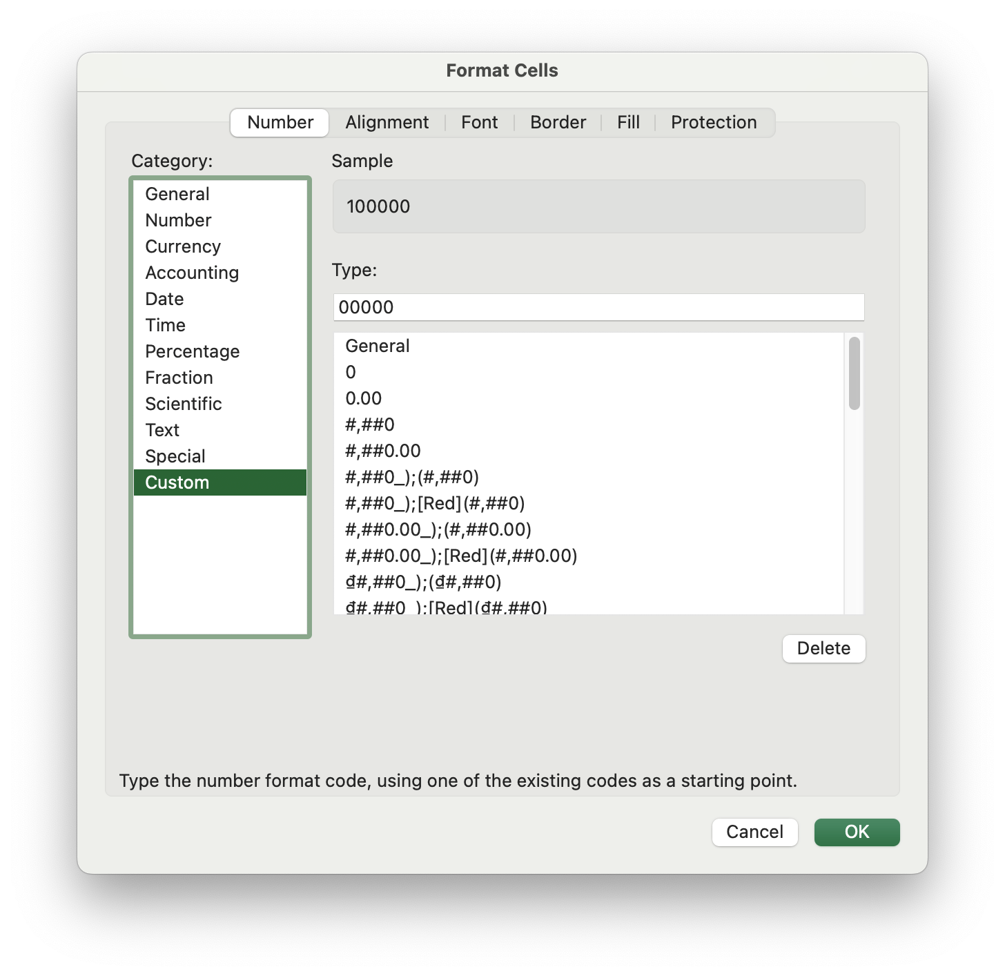
#6: CUSTOM – Tuỳ chỉnh
Một số định dạng cơ bản trong thẻ CUSTOM:
Some formattings in CUSTOM page:
| Loại | Dữ liệu Text | Dữ liệu Value |
|---|---|---|
| General | Hiển thị nguyên gốc | Hiển thị nguyên gốc |
| 0 | Không hỗ trợ | Hiển thị số nguyên (0.25 -> 0) |
| 0.00 0.000 Có thể nhập bao nhiêu số 0 tuỳ nhu cầu | Không hỗ trợ | Hiển thị 2 số thập phân (1 -> 1.00) Hiển thị 3 số thập phân (1 -> 1.000) Hiển thị n số thập phân (1 -> 1.n) |
| #,##0 | Không hỗ trợ | Phân cách hàng nghìn (5000 -> 5,000) |
| #,##0.00 | Không hỗ trợ | Phân cách hàng nghìn và thêm 2 số thập phân (2000 -> 2,000.00) |
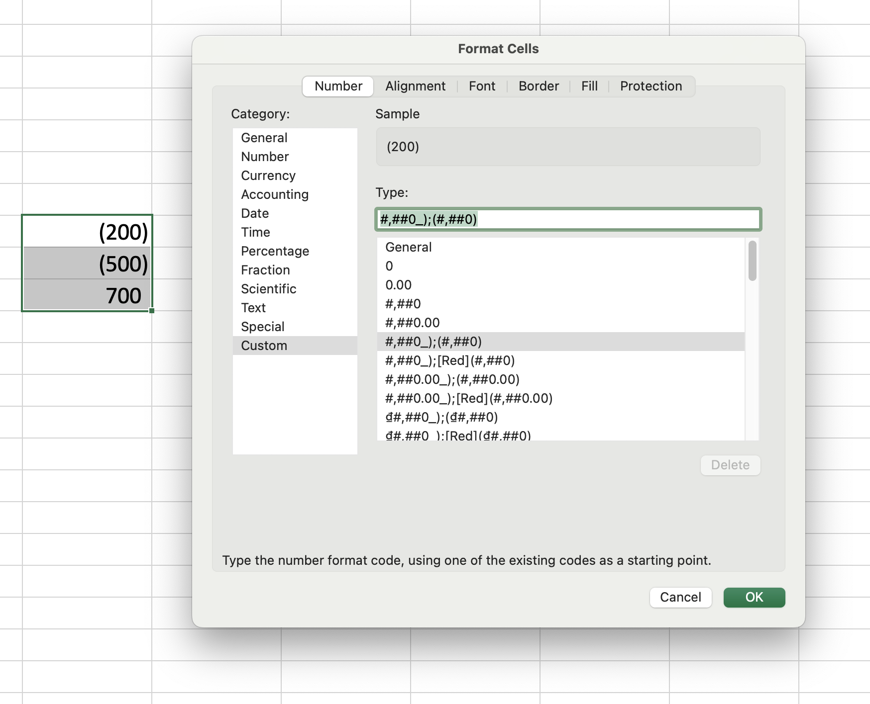
| #,##0_);(#,##0) | Không hỗ trợ | _) Excel sẽ thêm một khoảng trống rộng bằng dấu ngoặc ) để đảm bảo số âm và số dương canh đều nhau |
| Type | Text | Value |
|---|---|---|
| General | Show the original value | Show the original value |
| 0 | Not supported | Convert to a integer (0.25 -> 0) |
| 0.00 0.000 Có thể nhập bao nhiêu số 0 tuỳ nhu cầu | Not supported | Display 2 decimal places (1 -> 1.00) Display 3 decimal places (1 -> 1.000) Display 4 decimal places (1 -> 1.n) |
| #,##0 | Not supported | Use Thousands separator (5000 -> 5,000) |
| #,##0.00 | Not supported | Use Thousands separator and display 2 decimal places (2000 -> 2,000.00) |
| #,##0_);(#,##0) | Not supported | _) Excel will leave a space the width of a parenthesis character at the end of positive numbers. This ensures that positive and negative numbers align nicely when negative numbers are wrapped in parentheses. |
Mở rộng CUSTOM – More about CUSTOM:
Dữ liệu nhập vào trong Excel thuộc 1 trong 4 trường hợp như bản dưới:
Input in Excel belongs to one of four cases as the following table:
| Số dương (+); | Số âm (-); | Số 0; | Chữ |
| Positive (+) | Negative (-) | Zero; | Text |
Yêu cầu 1: Nhập dữ liệu bất kỳ vào Excel, nếu nhập vào số dương sẽ hiển thị thêm dấu + (cộng) phía trước, nếu là số âm hiển thị thêm dấu – (trừ) phía trước, nếu là số 0 sẽ hiển thị chữ “không” và nếu là chữ sẽ không hiển thị gì (“”).
Task 1: Input randomly a value into Excel cell. If it is a positive number, the cell display a plus sign (+) at the left of the number, esle add a minus sign (-). Or if it is 0, display “zero” and show nothing (“”) if it is any text.
Format như sau:
Format as follow:
| Số dương (+); | Số âm (-); | Số 0; | Chữ |
| “+”General; | “-“General; | “không”; | “” |
Trong đó:
• các dấu + (cộng), – (trừ) và chữ không phải nằm trong hai dấu ” ” (nháy kép),
• “” không hiển thị gì,
• Nếu yêu cầu phân cách hàng nghìn sẽ thay số 0 thành #,##0, hoặc thêm hai số thập phân thì thay thành 0.00
At which:
• plus and minus signs have to put between ” ” (quotation marks),
• “” display nothing in a cell,
• Replace 0 with #,##0 or 0.00 if required.
Yêu cầu 2: Nếu nhập vào số dương sẽ hiển thị màu xanh dương, nếu là số âm hiển thị màu đỏ, nếu là số 0 và chữ sẽ không đổi màu
Task 2: Display a cell in blue if the value is positive, esle red if negative. Display the default color if 0.
| Số dương (+); | Số âm (-); | Số 0; | Chữ |
| [Blue]General; | [Red]General; | General; | General |
Màu sắc sẽ được viết bằng tiếng Anh và nằm giữa hai dấu [ ] (ngoặc vuông).
Colors is in English and put between [ ] (breakets)
8 màu được sử dụng theo Visual Basic colors – Some main colors:
[Black], [Blue], [Cyan], [Green], [Magenta], [Red], [White], [Yellow]

Bên cạnh màu sắc, có thể thêm các icon thể hiện sự tăng, giảm hay đi ngang (0) như ▼,▲ , ↔ hoặc những icon khác tuỳ sở thích của bạn:
Additionally, add some icons like ▼,▲ , ↔ to display the trend of numbers:
| +; | –; | 0; | Text |
| [Blue]”▲”General; | [Red]”▼”General; | “↔”0; | General |
#6.1: Phone Number – Số điện thoại
Khi nhập số điện thoại, Excel sẽ mặc định bỏ số 0 phía trước vì nó không có nghĩa (trừ những số thập phân nằm trong đoạn (0;1))
Excel do not display 0 at the left of numbers (except from decimals between o and 1)
Cách 1: Chỉ cần gõ thêm phím cách giữa các thành phần, số sẽ chuyển sang dạng text nên vẫn giữ được số 0, ví dụ: 0905 12345, hoặc 0905 123 456.
Solution 1: Add a space between two parts of a phone number, ex: 0905 123456 or 0905 123 456.
Cách 2: Dùng dấu ‘ (nháy đơn) để tắt tính năng số, dữ liệu chuyển sang dạng text nên vẫn giữ được số 0, ví dụ: ‘0905123456
Solution 2: Add a sign ‘ (apostrophe) to convert a number to a text then Excel will keep 0 at the left of numbers, ex: ‘0905123456
Cách 3: Trong thẻ CUSTOM, nhập thêm số 0 phía trước định dạng, ví dụ: “0”0 hoặc “0”General.
Solution 3: In CUSTOM page, add a 0 number at the left of a codes, ex: “0”0 or “0”General.
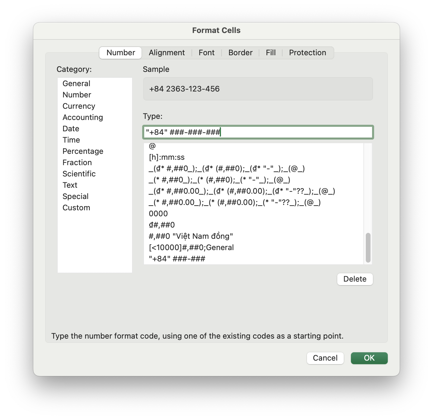
#6.2: Phone Number with region code- Số điện thoại có mã vùng
| Tỉnh Thành – Province/City | Mã Vùng – Region Code |
| An Giang | 296 |
| Bà Rịa – Vũng Tàu | 254 |
| Bắc Cạn | 209 |
| Bắc Giang | 204 |
| Bạc Liêu | 291 |
| Bắc Ninh | 222 |
| Bến Tre | 275 |
| Bình Định | 256 |
| Bình Dương | 274 |
| Bình Phước | 271 |
| Đà Nẵng | 236 |
| … | … |
Nhập định dạng “+84” ###-###-### tại thẻ Custom:
Enter the code “+84” ###-###-### at the Custom page:
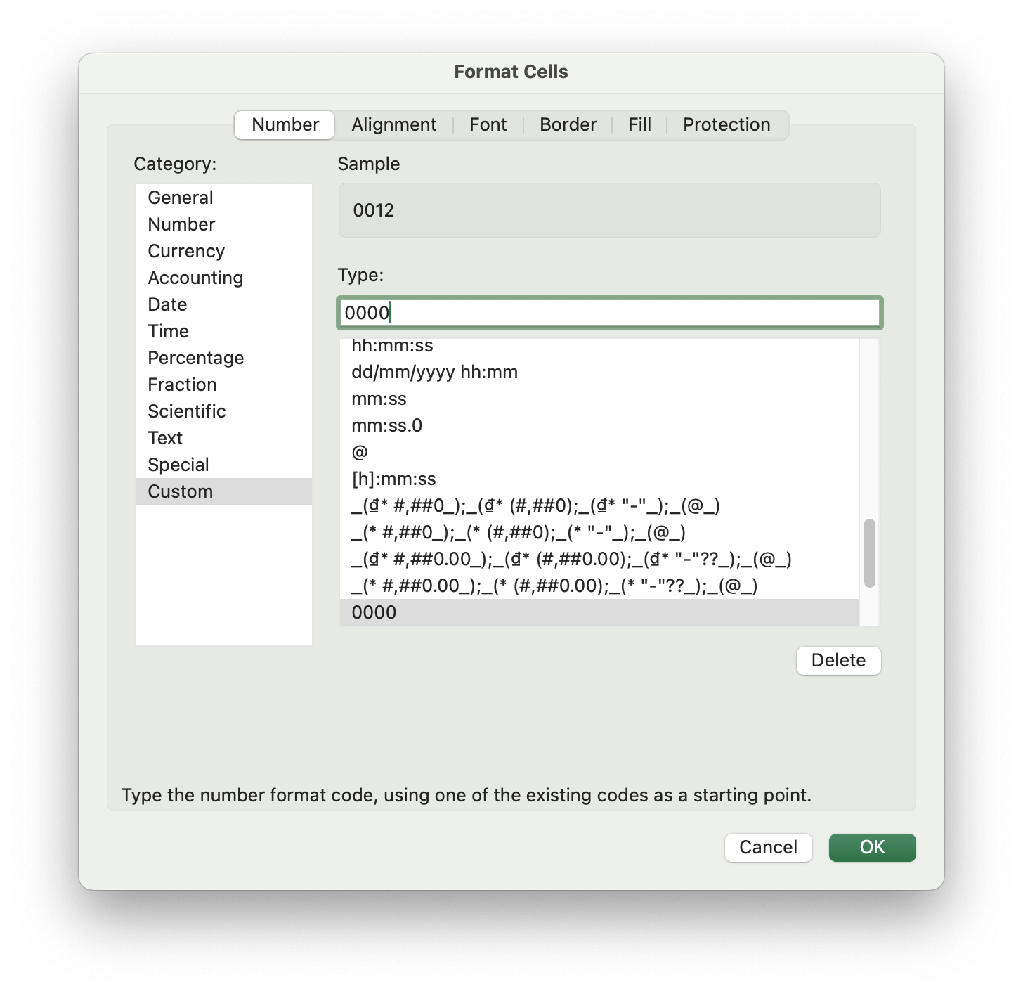
#6.3: Candidate Number – Số báo danh
Nhập định dạng 000 (hoặc 0000, 00000 tuỳ nhu cầu):
Type 000 (or 0000, 00000):
#6.3: Thousands, Millions, Billions, Trillions – Hàng ngàn, hàng triệu, hàng tỷ, hàng ngàn tỷ
Tại thẻ custom, nhập định dạng như sau:
At the custom tab, enter the formats as following:
| Number | Syntax | Comma Style | Shortened |
|---|---|---|---|
| Thousand | #,##0.00,\K (1 comma) | 157,645 | 157.65K |
| Million | #,##0.00,,\M (2 commas) | 75,230,000 | 75.23M |
| Billion | #,##0.00,,,\B (3 commas) | 450,235,000,000 | 450.24B |
| Trillion | #,##0.00,,,,\T (4 commas) | 654,460,000,000,000 | 654.46T |
#6.4: Set Limitations – Thiết lập điều kiện
Thiết lập điều kiện cho giá trị phải lớn/nhỏ hơn một mức nào đó thì mới áp dụng định dạng này bằng cách đưa điều kiện ra đứng trước và phải bỏ trong ngoặc vuông.
Setting out a condition on a number which has to be greater/less than a number then is applied this custom by putting the condition before that number and wrapping it inside square brackets.

[>10000]#,##0: chỉ phân cách hàng nghìn cho các giá trị lớn hơn 10 nghìn.
Apply this format to only numbers greater than 10 thousand.
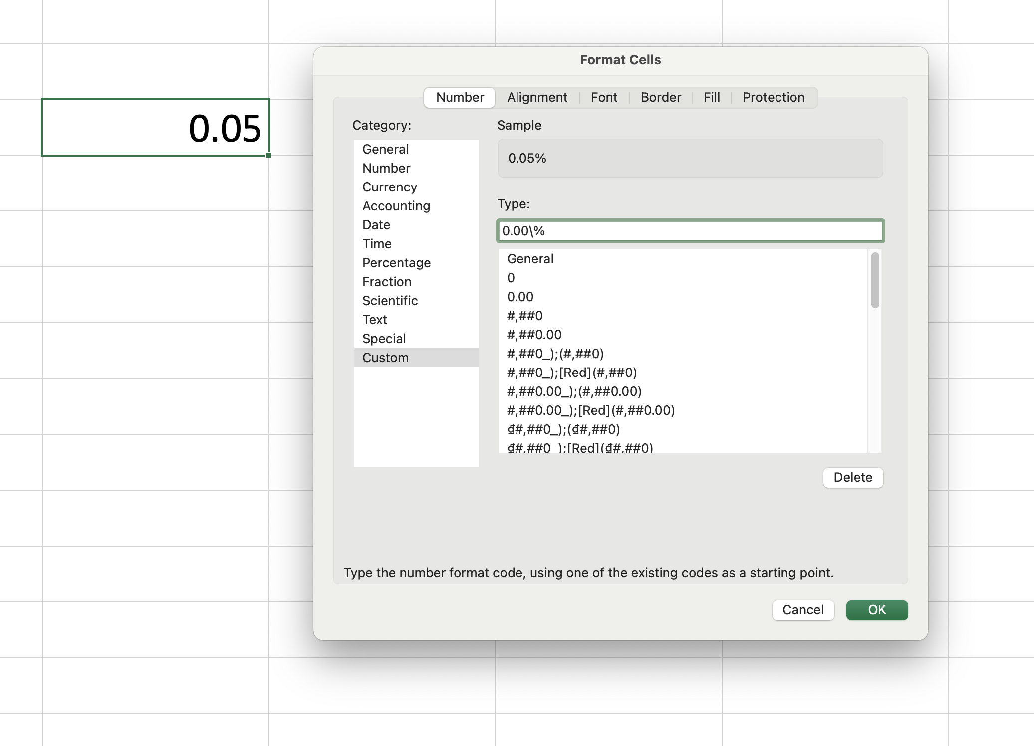
#6.5: Literal Character – Ký tự mang ý nghĩa hiển thị
Lấy ví dụ với số phần trăm. Khi chúng ta nhập vào 0.05 và tuỳ chỉnh định dạng là 0% tại Type Custom thì giá trị ban đầu 0.05 sẽ chuyển thành 5%, và dấu % lúc này có chức năng chuyển một số sang dạng phần trăm. Tuy nhiên, nếu chỉ muốn hiển thị ký hiệu % và nó không có chức năng chuyển đổi, thì chúng ta cần đặt dấu \ (backlash) đứng ngay trước %.
In the context of custom number formats in Excel, the backslash “\” is used as an escape character. It’s used to display a character that is typically used as a special character in a custom number format as a literal character instead. For example, in the format “0.00%”, the percentage sign “%” is a special character that indicates that the number should be displayed as a percentage. However, if you want to display the percentage symbol as a literal character and not as a special character, you can use the backslash as an escape character, like this: “0.00\%”. So, in the format “0.00\%”, Excel will display the percentage sign “%” as a literal character, and it won’t be treated as a special character for formatting purposes.
#6.6: Asterisk in Currency – Dấu hoa thị trong định dạng tiền tệ
Dấu hoa thị (*) đứng ngay sau ký hiệu tiền tệ mang ý nghĩa: ký hiệu tiền tệ sẽ được căn lề trái của cô, phần số còn lại vẫn giữ nguyên căn lề phải. Điều này giúp làm đẹp về phần nhìn cho các ô chứa giá trị tiền tệ.
The asterisk (*) is indeed used to ensure that the currency symbol aligns with the left border of the cell, and the numbers align with the right border of the cell. This is commonly used to improve the visual alignment of currency values in Excel.
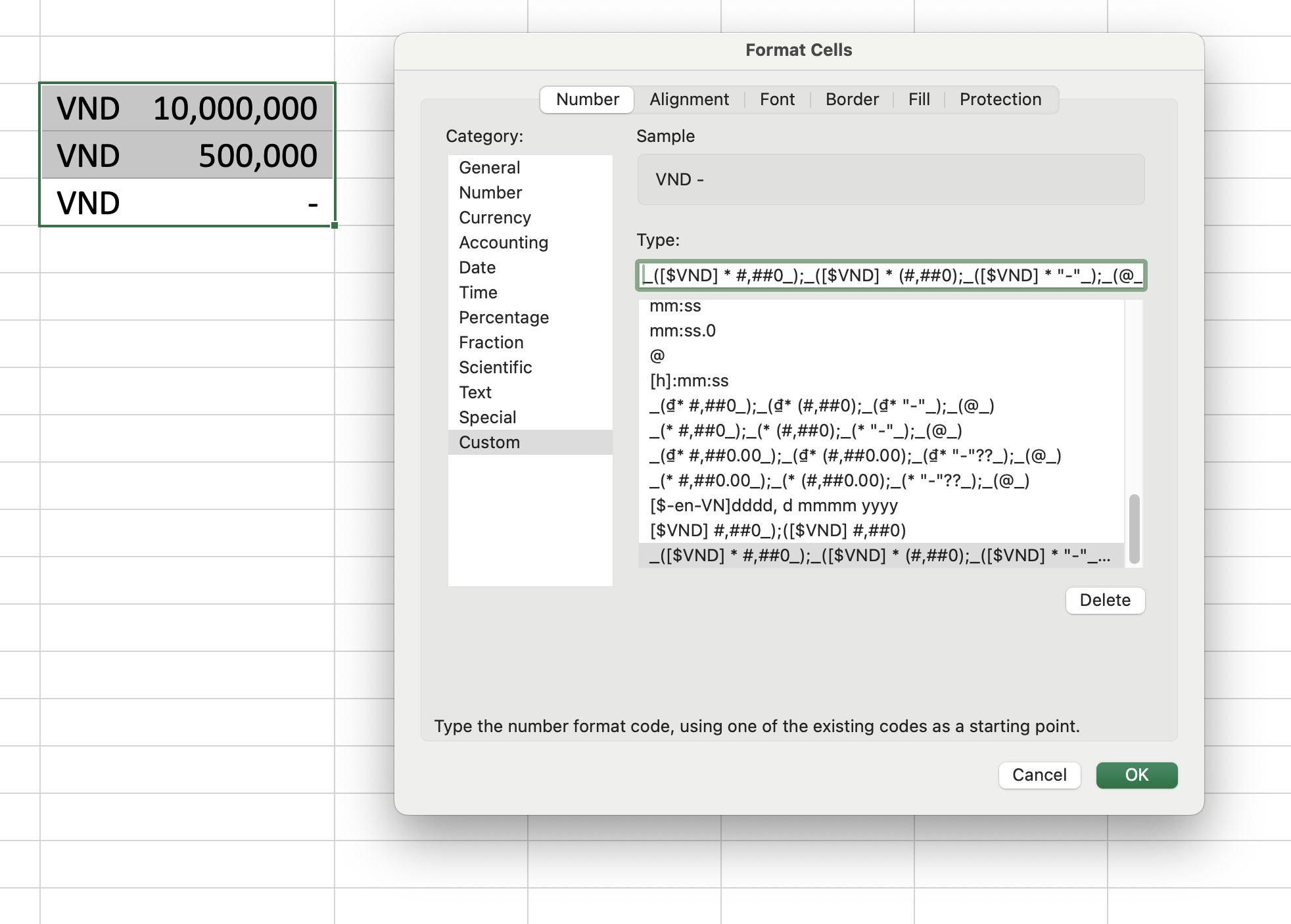
Khi định dạng không chứa dấu hoa thị ngay sau ký hiệu tiền tệ, thì đơn vị này sẽ hiển thị ngay bên trước số tiền. Định dạng này đơn giản dễ nhớ, nhưng vì đơn vị tiền tệ không ngay hàng với nhau nên có thể sẽ gây khó khăn cho người đọc.
When you format currency values in Excel without using the asterisk, the currency symbol is displayed once before the entire number. This formatting is simple and clear but may result in the currency symbol being misaligned with the numbers, especially when dealing with larger values.
#6.7: At symbol – Dấu @
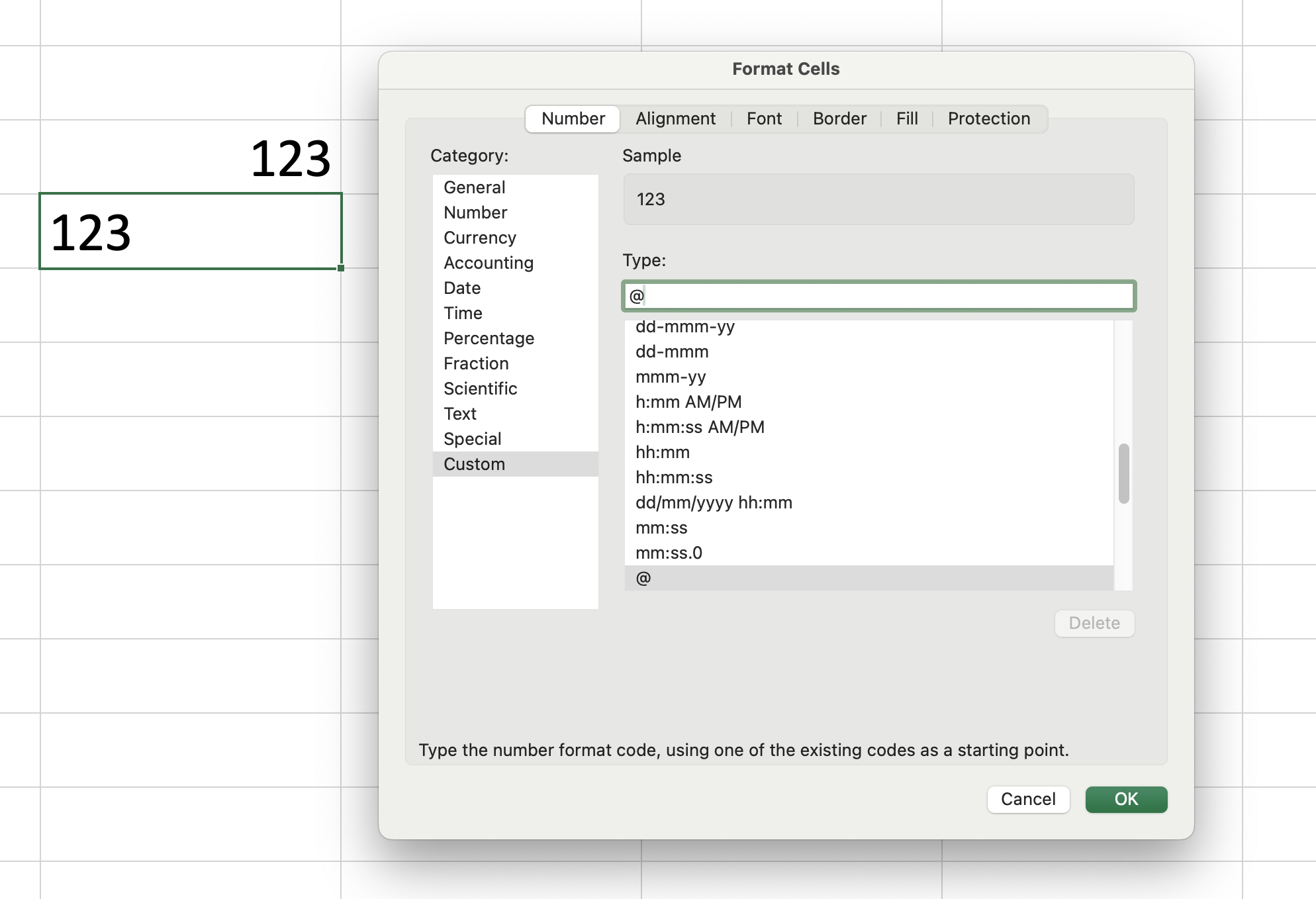
Dấu @ trong Custom có hai công dụng chính: dấu này sẽ giữ nguyên định dạng mặc định của dữ liệu dạng text (không phải number) and chuyển đổi trạng thái từ number sang text. Khi gõ @ vào Type Custom, Excel sẽ hiển thị dữ liệu đúng với những gì chúng ta gõ vào ô đó, bỏ qua kiểu dữ liệu đó là gì.
The “@” symbol in Excel’s custom number formatting serves a dual purpose: it both preserves the original formatting of non-numeric data and transforms numeric data into text. When you apply the “@” format to a cell, it essentially tells Excel to display the cell’s content exactly as entered, regardless of its data type.
#6.8: Special elements in Date format – Thành phần đặc biệt trong định dạng Ngày
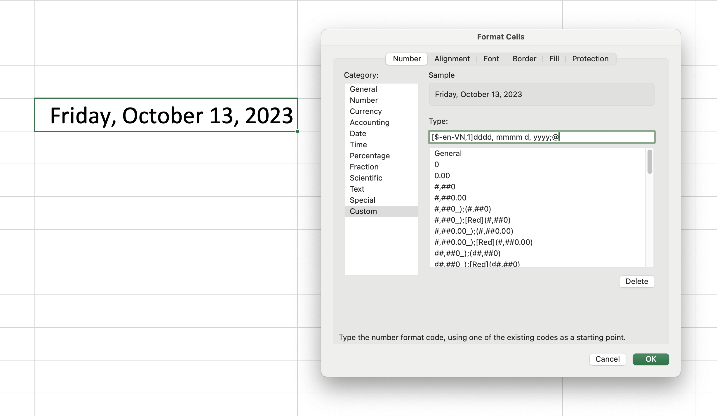
[$-en-VN,1]: Tổ hợp các ký tự này đại diện cho ngôn ngữ, vùng, và định dạng hệ thống thời gian (ngày).
• $: mở đầu cho một định dạng quốc tế, thường gặp trong thời gian, tiền tệ;
• en: ngôn ngữ hiển thị là tiếng Anh;
• VN: Excel sẽ định dạng thời gian dựa theo khu vực cụ thể, trong trường hợp này là Việt Nam;
• 1: hệ thống thời gian, số 1 chỉ hệ thống 1990 (WinOS – mặc định), số 2 chỉ hệ thống 1904 (MacOS – hệ thống này giả thiết không có năm nhuận trong 1900 và được sử dụng trong một số phiên bản Excel hoạt động trên MacOS, hệ thống này tính toán thời gian chính xác hơn nhưng không phổ biến trên WinOS).
This part of the format specifies the language, locale, and date system to be used for formatting. Here’s what each component means:
• $: an opening element of international formats, such as date or currency;
• en: This represents the English language. It indicates that the format is specified in English;
• VN: This represents the Vietnamese locale. It instructs Excel to format dates according to the conventions and language specific to Vietnam;
• 1: This is the date system identifier. It specifies the 1900 date system, which is the default date system in Excel. It affects date calculations and how dates are stored internally. Number 2 – this system assumes there was no leap year in 1900 and is used in some Mac versions of Excel. It is more accurate in terms of date calculations but less common in Windows versions;
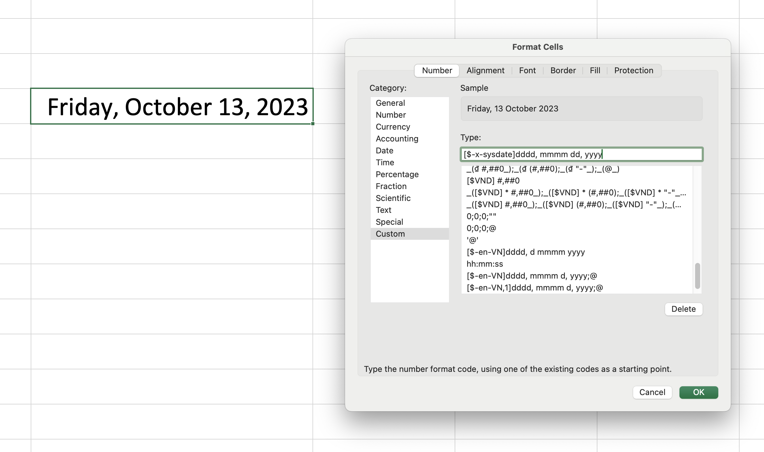
x-sysdate: chỉ ra rằng ngày sẽ được hiển thị theo khu vực của hệ thống
This syntax specifies that the date should be displayed in the system’s locale.
Tham khảo thêm tại đây.
Learn more.
Your message has been sent

